AP Calculus AB and BC

AP Calculus AB and BC Formula Sheet

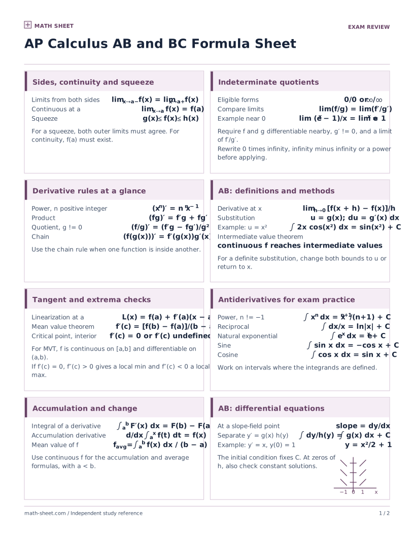
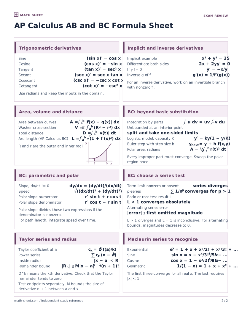
Use page 1 for core AB methods, then use page 2 for additional formulas and marked BC extensions. This Math Sheet printable is an independent practice reference. Check College Board for course and exam information.

This is an independent Math Sheet study resource for preparation. See the exam provider’s resources below.

On this page

Find a formula

Open a formula for its definition and a worked example.

Limits and function behavior

  • Compare nearby values and the value at the pointlim x→a f(x) = L, continuity requires L = f(a)For a two-sided limit, the left and right limits must agree.

    What it does

    A two-sided limit measures the value approached from both sides. Continuity at a point additionally requires that the function be defined there at the limiting value.

    Worked example

    Let f(x) = (x² − 9)/(x − 3) for x ≠ 3 and f(3) = 5. Find the limit at 3 and test continuity.

    1. Cancel x − 3 away from 3 to get x + 3, so both sides approach 6.
    2. The limit is 6, which differs from 5. The function is discontinuous at 3.
    Link to this example
  • Find an intermediate outputIf f is continuous on [a, b], every value between f(a) and f(b) equals f(c) for some c in [a, b].

    What it does

    The Intermediate Value Theorem guarantees that a continuous function on a closed interval takes every value between its endpoint outputs.

    Worked example

    Show that x³ + x = 1 has a solution between 0 and 1.

    1. The polynomial is continuous, and its values at 0 and 1 are 0 and 2.
    2. Since 0 < 1 < 2, some c in (0, 1) satisfies c³ + c = 1.
    Link to this example
  • Basic small-angle limitlim x→0 (sin x)/x = 1Measure x in radians.

    What it does

    In radians, sine and the angle itself approach zero at the same rate, so their ratio approaches 1.

    Worked example

    Evaluate lim x→0 sin(4x)/x.

    1. Multiply and divide by 4 to write 4·sin(4x)/(4x).
    2. As 4x tends to zero, the ratio tends to 1 and the limit is 4.
    Link to this example
  • Resolve a 0/0 or ∞/∞ limitlim f/g = lim f′/g′Use differentiable numerator and denominator near the limit point with g′ ≠ 0 there. The derivative quotient must approach a finite or infinite limit.

    What it does

    L’Hôpital’s rule replaces a qualifying 0/0 or ∞/∞ quotient with the quotient of separate derivatives near the limit point, if the new limit exists.

    Worked example

    Evaluate lim x→0 (e3x − 1)/x.

    1. Both expressions tend to zero, and the derivative of the denominator is 1.
    2. The derivative quotient is 3e3x, whose limit is 3.
    Link to this example
See Limits Cheat Sheet

Derivative rules and implicit equations

  • Compute the slope as a limitf′(x) = lim h→0 (f(x + h) − f(x))/h

    What it does

    A derivative is the limit of secant slopes as the gap between input values approaches zero.

    Worked example

    Use the definition to find the derivative of f(x) = x² + x at x = 2.

    1. Compute [f(2 + h) − f(2)]/h = (5h + h²)/h for h ≠ 0.
    2. The quotient 5 + h tends to 5.
    Link to this example
  • Differentiate a power or product(xn)′ = nxn−1, (fg)′ = f′g + fg′Apply the power rule on an interval where the given power is differentiable. A constant has derivative zero.

    What it does

    The power rule differentiates a power on intervals where it is differentiable. The product rule differentiates each factor in turn while retaining the other.

    Worked example

    Differentiate x³(x² + 1) and check by expansion.

    1. The product rule gives 3x²(x² + 1) + x³(2x).
    2. Combine to get 5x⁴ + 3x², the derivative of x⁵ + x³.
    Link to this example
  • Differentiate a quotient or composition(f/g)′ = (f′g − fg′)/g², (f ∘ g)′(x) = f′(g(x))g′(x)For the quotient use g(x) ≠ 0.

    What it does

    The quotient rule divides a difference of cross products by the denominator squared. The chain rule multiplies the outer derivative at the inner input by the inner derivative.

    Worked example

    Differentiate (x² + 1)³/(x + 1).

    1. The numerator derivative is 3(x² + 1)²·2x by the chain rule.
    2. Apply the quotient rule to get [6x(x² + 1)²(x + 1) − (x² + 1)³]/(x + 1)² for x ≠ −1.
    Link to this example
  • Treat y as a function of xF(x, y) = 0 ⇒ Fx + Fy y′ = 0 ⇒ y′ = −Fx/FyThe explicit slope requires F_y ≠ 0.

    What it does

    Implicit differentiation treats y as a function of x. After differentiating both sides, solve for y′ where its coefficient is nonzero.

    Worked example

    Find the tangent slope to x² + y² = 25 at (3, 4).

    1. Differentiate to get 2x + 2yy′ = 0.
    2. Solve for y′ = −x/y, then substitute to get −3/4.
    Link to this example
See Derivatives cheat sheet

Derivatives of familiar functions

  • Trigonometric pairs(sin x)′ = cos x, (cos x)′ = −sin x, (tan x)′ = sec² x, (sec x)′ = sec x tan x, (csc x)′ = −csc x cot x, (cot x)′ = −csc² xUse radians and stay in the original domain.

    What it does

    These are the six derivatives of the basic trig functions on their original domains, with angles in radians.

    Worked example

    Differentiate sin x + cos x + tan x + sec x + csc x + cot x wherever all terms are defined.

    1. The first three give cos x − sin x + sec² x.
    2. The last three give sec x tan x − csc x cot x − csc² x. Add the two results.
    Link to this example
  • Exponentials and logs(ex)′ = ex, (ax)′ = ax ln a, (ln x)′ = 1/x, (loga x)′ = 1/(x ln a)Use a > 0 for an exponential. A real logarithm also needs a ≠ 1 and x > 0.

    What it does

    Exponential derivatives keep the exponential factor and multiply by the natural log of the base. A logarithm derivative divides by x and the natural log of its base.

    Worked example

    Differentiate ex + 2x + ln x + log2 x for x > 0.

    1. The two exponentials yield ex + 2x ln 2.
    2. Add the log derivatives 1/x + 1/(x ln 2).
    Link to this example
  • Inverse sine and inverse tangent(arcsin x)′ = 1/√(1 − x²), (arctan x)′ = 1/(1 + x²)The arcsine derivative needs |x| < 1.

    What it does

    Inverse trig derivatives give the rate of change of the output angle with respect to the input ratio. The arcsine derivative requires |x| < 1.

    Worked example

    Evaluate the derivative of arcsin x + arctan x at x = 1/2.

    1. The first derivative term is 1/√(1 − 1/4) = 2/√3.
    2. The second is 1/(1 + 1/4) = 4/5, giving 2/√3 + 4/5.
    Link to this example

Use a derivative to interpret a function

  • Find an instantaneous slope matching a secantf′(c) = (f(b) − f(a))/(b − a), a < c < bThe Mean Value Theorem requires continuity on [a, b] and differentiability on (a, b).

    What it does

    For a function continuous on a closed interval and differentiable inside, the Mean Value Theorem finds an interior derivative equal to the average slope.

    Worked example

    Find the Mean Value Theorem point for f(x) = x² on [1, 5].

    1. The secant slope is (25 − 1)/(5 − 1) = 6.
    2. Solve f′(c) = 2c = 6 to get c = 3.
    Link to this example
  • Identify and classify critical numbersAt a critical number c in the domain, f′(c) = 0 or f′(c) is undefined. At a stationary point, f″(c) > 0 gives a local minimum and f″(c) < 0 gives a local maximum.

    What it does

    A critical number lies in the function’s domain and has zero or undefined derivative. At a stationary point, a nonzero second derivative determines the type of extremum.

    Worked example

    Find and classify the critical number of f(x) = x² − 6x + 10.

    1. Set f′(x) = 2x − 6 equal to zero to get x = 3.
    2. Since f″(3) = 2 > 0, the function has a local minimum at 3.
    Link to this example
  • Read concavity on an intervalf″ > 0 ⇒ concave up, f″ < 0 ⇒ concave down

    What it does

    The sign of the second derivative describes how tangent slopes change across an interval.

    Worked example

    Find the concavity of f(x) = x³ − 12x on each side of 0.

    1. Differentiate twice to get f″(x) = 6x.
    2. The graph is concave down for x < 0 and concave up for x > 0.
    Link to this example
  • Approximate by the tangent lineL(x) = f(a) + f′(a)(x − a)Use x close to a.

    What it does

    Linearization uses the value and slope at a nearby input to approximate a function by its tangent line.

    Worked example

    Approximate √9.3 using a tangent line at x = 9.

    1. At 9 the square-root function is 3 and its derivative is 1/6.
    2. Add (1/6)·0.3 = 0.05 to get approximately 3.05.
    Link to this example

Antiderivatives and methods

  • Integrate a power∫ xn dx = xn+1/(n+1) + C for n ≠ −1, ∫ 1/x dx = ln|x| + CWork on an interval in the integrand’s domain.

    What it does

    Integrate an ordinary power by raising the exponent by one and dividing by the result. The exceptional exponent −1 integrates to ln|x| on an interval avoiding zero.

    Worked example

    Integrate 6x² + 2/x for x > 0.

    1. Use the power rule on 6x² to get 2x³.
    2. The reciprocal contributes 2 ln x, so the result is 2x³ + 2 ln x + C.
    Link to this example
  • Exponential, sine and cosine∫ ex dx = ex + C, ∫ sin x dx = −cos x + C, ∫ cos x dx = sin x + C

    What it does

    Antiderivatives undo differentiation. The natural exponential reproduces itself, while sine and cosine integrate to negative cosine and sine respectively.

    Worked example

    Integrate 2ex − 3 sin x + cos x.

    1. The first two terms contribute 2ex and 3 cos x.
    2. Add sin x and the integration constant to get 2ex + 3 cos x + sin x + C.
    Link to this example
  • Undo a chain ruleu = g(x), du = g′(x) dx, so ∫ f(g(x))g′(x) dx = ∫ f(u) du

    What it does

    Substitution undoes a chain rule when the integrand has an inner expression and a matching derivative factor.

    Worked example

    Evaluate ∫ 6x(x² + 4)² dx.

    1. Let u = x² + 4, so du = 2x dx and the integral becomes ∫ 3u² du.
    2. Integrate to get u³ + C = (x² + 4)³ + C.
    Link to this example
  • Undo a product rule∫ u dv = uv − ∫ v duIntegration by parts is a BC review topic.

    What it does

    Integration by parts undoes the product rule by moving a derivative to another factor. It is an AP Calculus BC technique.

    Worked example

    Evaluate ∫ x cos x dx.

    1. Choose u = x and dv = cos x dx. Then du = dx and v = sin x.
    2. Subtract ∫ sin x dx from x sin x to get x sin x + cos x + C.
    Link to this example
See Integral Table and Integration Formulas

Accumulation and geometric applications

  • Differentiate accumulation or evaluate net changed/dx ∫ax f(t) dt = f(x), ∫ab f′(x) dx = f(b) − f(a)Use continuous integrands for these standard forms.

    What it does

    The Fundamental Theorem makes continuous accumulation differentiable at the moving endpoint and evaluates the integral of a derivative by its net change.

    Worked example

    Find d/dx ∫0x (3t² + 1) dt and evaluate the same integral at x = 2.

    1. The derivative is 3x² + 1 by continuity of the integrand.
    2. Evaluate t³ + t at 2 and 0 to get 10.
    Link to this example
  • Average height or enclosed areafavg = (∫ab f(x) dx)/(b − a), A = ∫ab [upper(x) − lower(x)] dxSplit an area integral where the curves cross.

    What it does

    Average value divides signed accumulation by interval length. Geometric area between curves integrates the upper height minus the lower height.

    Worked example

    Find the average of f(x) = x² on [0, 2] and the area between f and g(x) = 0 on that interval.

    1. Integrate x² to get 8/3. Here f ≥ g, so this is also the area.
    2. Divide by the interval length 2 to get average value 4/3.
    Link to this example
  • Integrate cross-sectional areaV = ∫ab A(x) dx. For washers, A(x) = π[R(x)² − r(x)²].R and r are distances to the axis of rotation. A disk has r = 0.

    What it does

    Integrating cross-sectional area gives volume. A washer is the difference of two disks with radii measured from the rotation axis, and a disk has no hole.

    Worked example

    Rotate the region 1 ≤ y ≤ x on 1 ≤ x ≤ 2 around the x-axis. Find the volume.

    1. The washer has R = x and r = 1, so A(x) = π(x² − 1).
    2. Evaluate π[x³/3 − x] from 1 to 2 to get 4π/3.
    Link to this example
  • Integrate cylindrical shells as enrichmentV = 2π ∫ab radius(x) × height(x) dxFor rotation about the y-axis with 0 ≤ a < b and region under f ≥ 0, use radius x and height f(x).

    What it does

    The shell method integrates the product of circumference and height. It is enrichment on this AP review.

    Worked example

    Rotate 0 ≤ y ≤ 2x for 0 ≤ x ≤ 1 around the y-axis using shells.

    1. A shell at x has radius x and height 2x. The integrand is 2πx·2x.
    2. Integrating 4πx² from 0 to 1 gives 4π/3.
    Link to this example
  • Measure the length of a smooth graphL = ∫ab √(1 + [f′(x)]²) dxArc length is a BC topic.

    What it does

    For a smooth graph, the arc length integral adds the lengths of infinitesimal horizontal and vertical displacements. This is a BC topic.

    Worked example

    Find the length of y = 3x − 1 for 0 ≤ x ≤ 2.

    1. The constant derivative 3 gives arc length integrand √(1 + 9) = √10.
    2. Integrate this constant across an interval of length 2 to get 2√10.
    Link to this example

BC curves given by a parameter or angle

  • Track position, slope and speedr(t) = ⟨x(t), y(t)⟩, dy/dx = y′(t)/x′(t), speed = √(x′(t)² + y′(t)²)The slope formula needs x′(t) ≠ 0.

    What it does

    A position vector records both coordinates as functions of time. Velocity is its derivative, speed is the magnitude, and slope is the velocity component ratio when horizontal velocity is nonzero.

    Worked example

    For r(t) = ⟨3t, t²⟩, find position, slope and speed at t = 2.

    1. Position is ⟨6, 4⟩ and velocity is ⟨3, 4⟩.
    2. The slope is 4/3 and speed is √(3² + 4²) = 5.
    Link to this example
  • Integrate speed to find arc lengthL = ∫ab √(x′(t)² + y′(t)²) dt

    What it does

    Parametric arc length is the integral of speed over the parameter interval.

    Worked example

    Find the length of x(t) = 5t, y(t) = 12t for 0 ≤ t ≤ 3.

    1. The coordinate derivatives are 5 and 12, giving speed 13.
    2. Multiply the constant speed by interval length 3 to get arc length 39.
    Link to this example
  • Sweep a polar region onceA = (1/2) ∫αβ r(θ)² dθ

    What it does

    Polar area adds sector slices over angles in radians. Choose bounds that cover the region once.

    Worked example

    Find the area swept by r = 3 over 0 ≤ θ ≤ π/3.

    1. The integrand in the polar area formula is 3²/2 = 9/2.
    2. Multiply by the angle width π/3 to get 3π/2.
    Link to this example
  • Differentiate polar coordinates separatelydy/dx = (r′ sin θ + r cos θ)/(r′ cos θ − r sin θ)The denominator is dx/dθ and must be nonzero.

    What it does

    For a polar curve, convert x = r cos θ and y = r sin θ, then take the quotient of their derivatives where dx/dθ is nonzero.

    Worked example

    Find the tangent slope for r = 2 at θ = π/4.

    1. Here r′ = 0, so dy/dθ = 2 cos θ and dx/dθ = −2 sin θ.
    2. At π/4 these have equal magnitudes and opposite signs, so the slope is −1.
    Link to this example

BC series and approximation

  • Two standard infinite sumsΣn=0∞ arn = a/(1 − r) if |r| < 1. Σn=1∞ 1/np converges exactly when p > 1.

    What it does

    A nonzero geometric series converges if its ratio has magnitude below one. A p-series beginning at one converges precisely when p > 1.

    Worked example

    Sum 3 + 1 + 1/3 + … and classify Σn=1∞ 1/n3/2.

    1. The geometric ratio is 1/3, so the sum is 3/(1 − 1/3) = 9/2.
    2. The second series has p = 3/2 > 1 and therefore converges.
    Link to this example
  • Compare successive magnitudesL = lim n→∞ |an+1/an|L < 1 gives absolute convergence, L > 1 gives divergence, and L = 1 is inconclusive.

    What it does

    The ratio test checks the limiting magnitude of one term divided by the previous one. A limit below one gives absolute convergence and one gives no decision.

    Worked example

    Test Σn=1∞ 4n/n! for convergence.

    1. The absolute ratio of consecutive terms is 4/(n + 1).
    2. It approaches zero, so the series converges absolutely.
    Link to this example
  • Build a Taylor series at aΣn=0∞ f(n)(a)(x − a)n/n!It equals f(x) where the Taylor remainders tend to zero.

    What it does

    Taylor coefficients are derivatives at the center divided by factorials. The series equals the original function where the Taylor remainders tend to zero.

    Worked example

    Find the degree-two Taylor polynomial for f(x) = x³ centered at 1.

    1. The derivatives of orders 0, 1 and 2 at 1 are 1, 3 and 6.
    2. Divide by 0!, 1! and 2! to get 1 + 3(x − 1) + 3(x − 1)².
    Link to this example
  • Three series centered at zeroex = Σn=0∞ xn/n!, sin x = Σn=0∞ (−1)n x2n+1/(2n+1)!, cos x = Σn=0∞ (−1)n x2n/(2n)!All three converge for every real x.

    What it does

    The Maclaurin series for ex, sine and cosine expand around zero and converge on the entire real line. Sine uses odd powers, cosine uses even powers, and both alternate.

    Worked example

    Write the first three nonzero terms of each series.

    1. For ex the terms are 1 + x + x²/2.
    2. For sin x they are x − x³/6 + x⁵/120. For cos x they are 1 − x²/2 + x⁴/24.
    Link to this example
  • Bound the Taylor approximation error|Rn(x)| ≤ M|x − a|n+1/(n+1)!Choose M to bound the magnitude of the derivative of order n + 1 between a and x.

    What it does

    The Lagrange bound controls Taylor error using the largest possible magnitude of the next derivative between the center and target.

    Worked example

    Bound the error of approximating cos(0.1) by 1 − (0.1)²/2.

    1. The polynomial has degree 2 at zero. The third derivative of cosine is sin x, bounded in magnitude by 1.
    2. Thus |error| ≤ 1·(0.1)³/3! = 1/6000.
    Link to this example
See Sequences and Series Formula Sheet

Preview the printable

Download the compact sheet for a quick review, or print the complete formula list from this page.

Practice these skills

Related references

Sources and review

Math Sheet prepares original print materials. See how we check formulas and printouts.

Browse all formula sheets →