AP Statistics

AP Statistics Formula Sheet

Use this independent practice reference to choose a model or inference procedure and justify its conditions. For the exam format and official reference materials, use College Board’s AP Statistics page.

This is an independent Math Sheet study resource for preparation. See the exam provider’s resources below.

On this page

Find a formula

Open a formula for its definition and a worked example.

Center, spread and unusual values

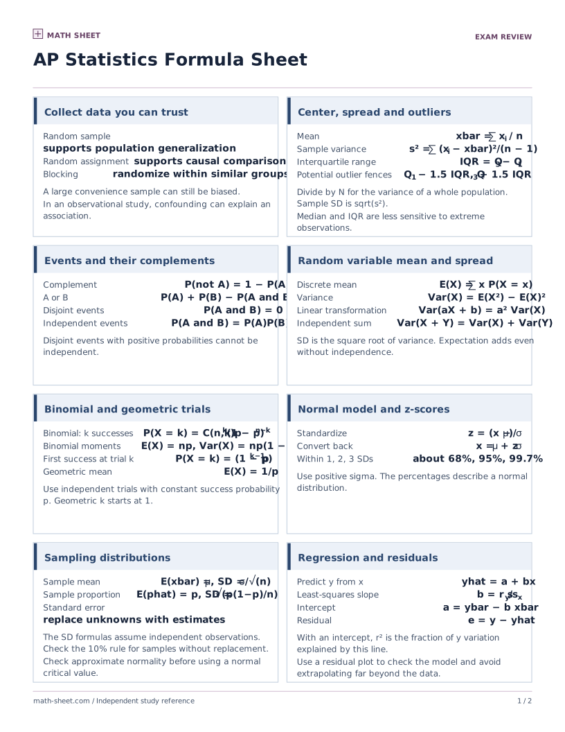
  • Summarize a samplex̄ = Σxi/n, s² = Σ(xi − x̄)²/(n − 1), s = √(s²)Sample variance needs n > 1.

    What it does

    The mean locates a sample’s center, variance measures squared deviations with n − 1 in the denominator, and standard deviation returns to the original units.

    Worked example

    Find x̄, s² and s for 2, 4 and 6.

    1. The mean is 4, giving squared deviations 4, 0 and 4.
    2. Divide 8 by n − 1 = 2 to get s² = 4, then take the square root to get s = 2.
    Link to this example
  • Count standard deviations from the meanz = (x − μ)/σAssume σ > 0.

    What it does

    A z-score expresses a value’s signed distance from the mean in standard-deviation units. The standard deviation must be positive.

    Worked example

    A quiz score is 72, with population mean 66 and standard deviation 3. Find z.

    1. Subtract the mean to get 6.
    2. Divide by 3 to get z = 2, or two standard deviations above the mean.
    Link to this example
  • Use quartiles to flag possible outliersIQR = Q₃ − Q₁, lower fence = Q₁ − 1.5 IQR, upper fence = Q₃ + 1.5 IQRFlag points strictly outside the fences.

    What it does

    The IQR is the width of the middle half of a distribution. The 1.5-IQR rule flags observations strictly beyond the fences.

    Worked example

    Given Q₁ = 8 and Q₃ = 14, flag any of −1, 0, 23 and 24.

    1. The IQR is 6, so the fences are 8 − 9 = −1 and 14 + 9 = 23.
    2. Only 24 is strictly beyond a fence. Values equal to a fence stay in.
    Link to this example

Combine or condition on events

  • Handle union and complementP(A ∪ B) = P(A) + P(B) − P(A ∩ B), P(Ac) = 1 − P(A)

    What it does

    A union counts outcomes in either event and subtracts their overlap once. A complement includes every outcome outside an event.

    Worked example

    For P(A) = 0.4, P(B) = 0.3 and P(A ∩ B) = 0.1, find P(A ∪ B) and P(Ac).

    1. Compute the union as 0.4 + 0.3 − 0.1 = 0.6.
    2. Subtract P(A) from 1 to get P(Ac) = 0.6.
    Link to this example
  • Multiply probabilities for independent eventsP(A ∩ B) = P(A)P(B)Use only when A and B are independent.

    What it does

    For independent events, learning whether one occurred leaves the probability of the other unchanged. Their joint probability is the product.

    Worked example

    A fair coin and a separate fair die are tossed. What is the probability of heads and an even roll?

    1. The two events each have probability 1/2 and are independent.
    2. Multiply the probabilities to get 1/4.
    Link to this example
  • Condition on an event with positive probabilityP(A | B) = P(A ∩ B)/P(B)The conditioning event B must have P(B) > 0.

    What it does

    Conditioning on an event restricts the sample space to its outcomes. Divide the joint probability by the positive probability of the conditioning event.

    Worked example

    Of 30 students, 12 cycle to school and 8 of those 12 carry a helmet. Find P(helmet | cycles).

    1. The cycling subgroup contains 12 students and the overlap contains 8.
    2. Divide 8/30 by 12/30 to get 2/3.
    Link to this example
  • Use Bayes’ rule to reverse the conditioningP(A | B) = P(B | A)P(A)/P(B)Require P(A) > 0 to define P(B | A) and P(B) > 0 to divide.

    What it does

    Bayes’ rule reverses the direction of conditioning using a prior and the probability of the evidence. Both conditioning events used must have positive probability.

    Worked example

    A factory makes 30% of its items on line A. Of A items 4% are defective. The overall defect rate is 2%. Find P(A | defective).

    1. The joint probability is 0.30·0.04 = 0.012.
    2. Divide by 0.02 to get 0.60.
    Link to this example
See Probability Formulas

Discrete means and variances

  • Weight by each outcome’s probabilityμ = Σ xi pi, σ² = Σ (xi − μ)² pi, σ = √(σ²)

    What it does

    A discrete random variable’s mean and variance weight each outcome and its squared deviation by its probability. The standard deviation is the square root of the variance.

    Worked example

    Let X = 0 or 4 with equal probabilities. Find its mean, variance and standard deviation.

    1. The mean is 0·0.5 + 4·0.5 = 2.
    2. The variance is 0.5·(−2)² + 0.5·2² = 4, and the standard deviation is 2.
    Link to this example
  • Shift or scale a random variableE[aX + b] = aE[X] + b, Var(aX + b) = a² Var(X)Optional general statistics reference.

    What it does

    In this optional extension, shifting a variable changes its mean and leaves its variance unchanged. Scaling multiplies the mean by the scale factor and variance by its square.

    Worked example

    If E[X] = 5 and Var(X) = 4, find the mean and variance of 3X − 2.

    1. Transform the mean to 3·5 − 2 = 13.
    2. Multiply the variance by 3² to get 36.
    Link to this example
  • Add independent variables as enrichmentVar(X + Y) = Var(X) + Var(Y)Combining random variables left the AP Statistics curriculum in 2026–27. In the general variance formula also add 2 Cov(X, Y).

    What it does

    The variance of a sum of independent variables equals the sum of their variances. Combining random variables is enrichment for the 2026–27 AP Statistics course.

    Worked example

    Two independent sensors have noise variances 4 and 9. Find the variance of their total noise.

    1. Independence gives covariance zero.
    2. The total variance is 4 + 9 = 13.
    Link to this example

Binomial, geometric and normal models

  • Count successes in n independent trialsP(X = k) = C(n,k)pk(1 − p)n−k, μ = np, σ = √(np(1 − p))The success probability p is fixed across trials and k runs from 0 to n.

    What it does

    A binomial variable counts successes in a fixed number of independent trials that share a success probability.

    Worked example

    Flip a fair coin four times. Find the probability of exactly one head, the mean and the standard deviation.

    1. Four choices for the head each have probability (1/2)⁴, giving 4/16 = 1/4.
    2. The mean is 4·(1/2) = 2 and the standard deviation is √(4·(1/2)·(1/2)) = 1.
    Link to this example
  • Geometric distribution as enrichmentP(X = k) = (1 − p)k−1p, μ = 1/pCounts trials until the first success, with independent trials, 0 < p ≤ 1 and k ≥ 1. This distribution left the AP Statistics curriculum in 2026–27.

    What it does

    A geometric variable counts the number of independent trials through the first success, including that success. It is enrichment for the 2026–27 AP Statistics course.

    Worked example

    Each free throw goes in independently with probability 1/4. Find P(first success on trial 3) and the expected wait.

    1. Two misses and a make have probability (3/4)²·(1/4) = 9/64.
    2. The mean number of throws is 1/(1/4) = 4.
    Link to this example
  • Standardize a normal variablef(x) = e−z²/2/(σ√(2π)), z = (x − μ)/σFor normal X and σ > 0, Z is standard normal with mean 0 and variance 1.

    What it does

    Standardization turns a normal variable into the standard normal by subtracting its mean and dividing by its positive standard deviation. Its density height differs from an event probability.

    Worked example

    Let X be normal with mean 50 and standard deviation 5. Find z and the density at x = 55.

    1. The z-score is (55 − 50)/5 = 1.
    2. Substitute into the density to get e−1/2/(5√(2π)).
    Link to this example

Spread of sample statistics

  • Sampling distribution of a meanE[X̄] = μ, SD(X̄) = σ/√n, estimated SE = s/√nWith independent sampling and finite variance, the mean is approximately normal for large n. It is exactly normal for a normal population.

    What it does

    A sample mean from independent observations has population mean μ and standard deviation σ/√n. The sample standard deviation can estimate that spread, and normality holds exactly for a normal population.

    Worked example

    Take 25 independent observations from a normal population with μ = 30 and σ = 10. The sample has s = 8. Find the mean’s center, actual spread and estimated spread.

    1. The sampling mean is 30 and its standard deviation is 10/√25 = 2.
    2. The sample estimate of the standard error is 8/√25 = 1.6.
    Link to this example
  • Spread of a sample proportionSD(p̂) = √(p(1 − p)/n)This formula uses independent Bernoulli observations. Estimate it with p̂ when p is unknown and the procedure calls for an estimate.

    What it does

    A sample proportion is the average of independent Bernoulli outcomes. Its sampling spread depends on the true success probability and sample size.

    Worked example

    If p = 0.2 and n = 100 independent trials, find the standard deviation of p̂.

    1. Compute p(1 − p)/n = 0.2·0.8/100 = 0.0016.
    2. Take the square root to get 0.04.
    Link to this example
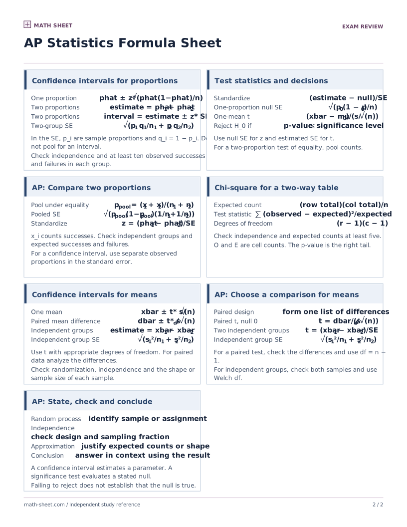
  • Estimated spread for a difference of independent meansSE = √(s₁²/n₁ + s₂²/n₂)

    What it does

    For independent samples, variances of the two mean estimates add, even when their means are subtracted.

    Worked example

    Two independent samples have n₁ = 16, s₁ = 8 and n₂ = 25, s₂ = 5. Estimate the spread of their mean difference.

    1. The two variance estimates are 8²/16 = 4 and 5²/25 = 1.
    2. Take the square root of their sum to get estimated standard error √5.
    Link to this example

Confidence intervals by parameter

  • Estimate one population meanx̄ ± z* σ/√n if σ is known, x̄ ± t* s/√n otherwiseFor the t interval use n − 1 degrees of freedom and check sample independence and the normality or large-sample condition.

    What it does

    A one-mean interval adds and subtracts a critical value times the standard error. Use z with known population spread, or t with estimated spread and n − 1 degrees of freedom.

    Worked example

    A suitable sample has mean 52 and n = 25. Find a 95% z interval if σ = 10 and a t interval if σ is unknown and s = 10. Use critical values 1.96 and 2.064.

    1. Both standard errors are 10/√25 = 2. The margins are 3.92 and 4.128.
    2. The intervals are (48.08, 55.92) and approximately (47.872, 56.128).
    Link to this example
  • Estimate one proportionp̂ ± z* √(p̂(1 − p̂)/n)Check independent observations and enough observed successes and failures.

    What it does

    A one-proportion z interval uses the observed proportion to estimate spread. Check independent observations and enough successes and failures.

    Worked example

    In an independent sample, 50 of 100 respondents choose A. Use 1.96 for a 95% interval.

    1. Compute p̂ = 0.5 and SE = √(0.5·0.5/100) = 0.05.
    2. The interval 0.50 ± 1.96·0.05 gives (0.402, 0.598).
    Link to this example
  • Estimate the difference of independent means(x̄₁ − x̄₂) ± t*√(s₁²/n₁ + s₂²/n₂)Use Welch’s degrees of freedom for the unpooled interval.

    What it does

    For independent samples, a two-mean t interval centers at the difference of the sample means and uses a combined standard error with an appropriate t critical value.

    Worked example

    For two suitable samples with x̄₁ = 40, x̄₂ = 36, s₁ = s₂ = 5 and n₁ = n₂ = 25, use t* = 2.011 for a 95% interval.

    1. The difference is 4 and SE = √(25/25 + 25/25) = √2.
    2. The interval 4 ± 2.011√2 is about (1.16, 6.84).
    Link to this example
  • Estimate the difference of independent proportions(p̂₁ − p̂₂) ± z*√(p̂₁(1 − p̂₁)/n₁ + p̂₂(1 − p̂₂)/n₂)Use each sample’s own estimate in the interval.

    What it does

    A difference-of-proportions interval uses the two observed rates separately to estimate spread. The samples must be independent and each rate must meet the count conditions.

    Worked example

    Two independent groups of 100 give proportions 0.60 and 0.40. Use 1.96 for a 95% interval.

    1. The difference is 0.20 and SE = √(0.24/100 + 0.24/100) ≈ 0.0693.
    2. The interval is 0.20 ± 1.96·0.0693, about (0.064, 0.336).
    Link to this example
See Statistics Formula Sheet

Test statistics against a null claim

  • Test one meanz = (x̄ − μ₀)/(σ/√n) or t = (x̄ − μ₀)/(s/√n)Use z if σ is known. For a one-sample t test use n − 1 degrees of freedom. For paired observations, compute each pair’s difference and run a one-sample t test on those differences.

    What it does

    A one-mean test measures how far the sample mean is from the null mean in standard errors. If observations are paired, perform a one-sample t test on the differences.

    Worked example

    To test μ₀ = 20, use an independent sample with mean 23 and n = 36. Compare the statistics when σ = 6 is known and when σ is unknown with s = 6.

    1. In both cases the standard error is 6/√36 = 1.
    2. The statistics are z = 3 and t = 3. Compare the latter with a t distribution with 35 degrees of freedom.
    Link to this example
  • Test one proportionz = (p̂ − p₀)/√(p₀(1 − p₀)/n)Use p₀ from the null hypothesis to calculate the spread.

    What it does

    A one-proportion z test computes its standard error using the null proportion, because the null is the model being tested.

    Worked example

    Test p₀ = 0.5 using 60 successes in 100 independent trials. Find z.

    1. Compute p̂ = 0.60 and null standard error √(0.5·0.5/100) = 0.05.
    2. Then z = (0.60 − 0.50)/0.05 = 2.
    Link to this example
  • Test homogeneity or independence in a two-way tableχ² = Σ (O − E)²/E, df = (rows − 1)(columns − 1)Check independence of observations and expected cell counts. Both two-way tests are in AP Statistics for 2026–27. The one-way goodness-of-fit test is an enrichment topic.

    What it does

    The chi-square statistic measures differences between observed and expected counts. The 2026–27 AP course includes homogeneity and independence for two-way tables.

    Worked example

    A two-by-two independence table has observed rows (30, 20) and (20, 30). Find χ² and degrees of freedom.

    1. All row and column totals are 50 and the grand total is 100, so each expected count is 25.
    2. Each cell contributes 25/25 = 1, giving χ² = 4 and (2 − 1)(2 − 1) = 1 degree of freedom.
    Link to this example
  • Test a difference of independent meanst = ((x̄₁ − x̄₂) − Δ₀)/√(s₁²/n₁ + s₂²/n₂)For the usual equal-means null hypothesis Δ₀ = 0.

    What it does

    A two-sample t statistic compares a difference of independent sample means with the null difference, using both samples’ variances to estimate spread.

    Worked example

    For independent samples with means 28 and 25, each with n = 16 and s = 4, test a null difference of zero. Find t.

    1. Compute SE = √(4²/16 + 4²/16) = √2.
    2. The statistic is (28 − 25 − 0)/√2 = 3/√2, about 2.12.
    Link to this example

Fit and interpret a regression line

  • Predict y from x by least squaresŷ = b₀ + b₁x, b₁ = r sy/sx, b₀ = ȳ − b₁x̄The slope requires variation in x.

    What it does

    A least-squares line predicts y from x. Its slope combines the correlation and relative spreads, and the line passes through the two sample means.

    Worked example

    Given x̄ = 8, ȳ = 14, sx = 2, sy = 5 and r = 0.8, predict y at x = 10.

    1. The slope is 0.8·5/2 = 2 and the intercept is 14 − 2·8 = −2.
    2. Use ŷ = −2 + 2x to predict 18.
    Link to this example
  • Relate correlation and explained variationr = Σ[(xi − x̄)/sx][(yi − ȳ)/sy]/(n − 1), R² = r²Both variables must vary. The identity for R² is for a simple linear regression with an intercept.

    What it does

    Correlation is the sum of the products of corresponding standardized scores divided by n − 1. In simple least-squares regression with an intercept, its square is the fraction of variation explained.

    Worked example

    For points (1, 2), (2, 4), (3, 6), find r and R².

    1. The standardized coordinates of each variable are −1, 0 and 1 in matching order.
    2. Their cross products sum to 2. Divide by 3 − 1 to get r = 1 and square to get R² = 1.
    Link to this example

Preview the printable

Download the compact sheet for a quick review, or print the complete formula list from this page.

Practice these skills

Related references

Sources and review

Math Sheet prepares original print materials. See how we check formulas and printouts.

Browse all formula sheets →