Introductory probability

Probability Formulas

Identify whether the question asks for an event, a conditional probability, a count or a random-variable model. The sheet puts each formula next to its assumptions.

On this page

Find a formula

Open a formula for its definition and a worked example.

Combine and complement events

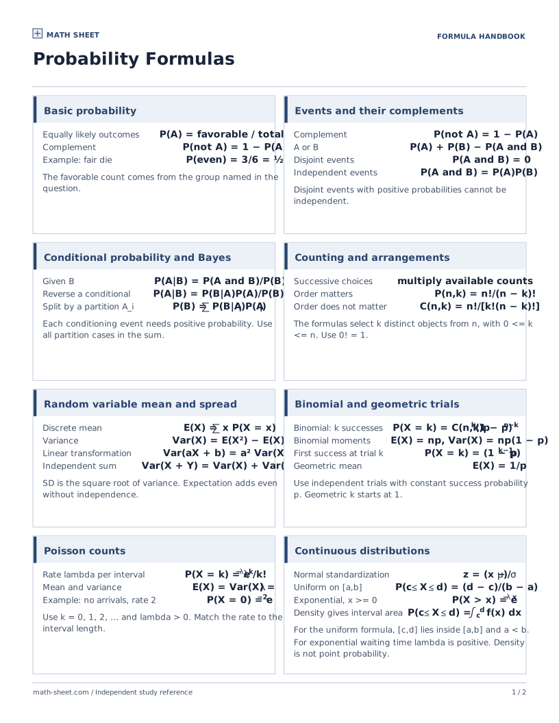
  • Count matching outcomesP(A) = outcomes in A / total outcomesUse a finite sample space of equally likely outcomes.

    What it does

    When a finite set of outcomes is equally likely, the probability of an event is its share of that set.

    Worked example

    A fair six-sided die is rolled. Find the chance of a value greater than 4.

    1. The favorable outcomes are 5 and 6, two of the six equally likely values.
    2. The probability is 2/6 = 1/3.
    Link to this example
  • Switch to the complementP(Aᶜ) = 1 − P(A)

    What it does

    An event and its complement cover all possible outcomes without overlap, so their probabilities total 1.

    Worked example

    A bus is on time with probability 0.86. Find the probability it is not on time.

    1. The complementary event takes the remaining probability.
    2. Subtract 0.86 from 1 to get 0.14.
    Link to this example
  • Find the chance of either eventP(A ∪ B) = P(A) + P(B) − P(A ∩ B)For disjoint events the intersection term is zero.

    What it does

    Adding the probabilities of two events counts their shared outcomes twice. Subtract the intersection once to obtain their union.

    Worked example

    On a fair die, A means even and B means at least 4. Find P(A ∪ B).

    1. Each event has probability 3/6, and their overlap {4,6} has probability 2/6.
    2. The union probability is 3/6 + 3/6 − 2/6 = 2/3.
    Link to this example
  • Find the chance of both eventsP(A ∩ B) = P(A)P(B | A). For independent events, P(A ∩ B) = P(A)P(B).The conditional form shown uses P(A) > 0.

    What it does

    For both events to occur, multiply the first probability by the chance of the second given the first. Independence makes this conditional chance equal to the ordinary second probability.

    Worked example

    Find the chance of two red draws from a bag with 3 red and 2 blue, first without replacement and then with replacement.

    1. Without replacement the chance is (3/5)(2/4) = 3/10.
    2. With replacement the draws are independent, giving (3/5)² = 9/25.
    Link to this example

Update probabilities with information

  • Restrict attention to BP(A | B) = P(A ∩ B)/P(B)Requires P(B) > 0.

    What it does

    Conditional probability rescales the sample space to outcomes where the given event occurred, provided that event has positive probability.

    Worked example

    For a fair die, what is the probability of even given the result is greater than 3?

    1. The given condition leaves {4,5,6}. Two of these three outcomes are even.
    2. The conditional probability is 2/3.
    Link to this example
  • Reverse a conditional probabilityP(A | B) = P(B | A)P(A)/P(B)Requires P(A) > 0 and P(B) > 0.

    What it does

    Bayes’ rule reverses the direction of conditioning by comparing a joint probability with the probability of the evidence.

    Worked example

    Factory A makes 60% of items and has a 2% defect rate. Factory B makes 40% and has a 5% defect rate. Given a defect, find the chance the item came from A.

    1. The joint probability for A and defect is 0.60 × 0.02 = 0.012. The total defect probability is 0.012 + 0.40 × 0.05 = 0.032.
    2. Divide 0.012 by 0.032 to obtain 0.375, or 37.5%.
    Link to this example
  • Sum over mutually exclusive casesP(B) = Σi P(B | Ai)P(Ai)The A_i form a partition of the sample space. Omit cases of zero probability.

    What it does

    The law of total probability adds the joint contribution from each mutually exclusive case in a partition of all outcomes.

    Worked example

    A weather model gives rain probability 0.3. The chance a game is canceled is 0.8 with rain and 0.1 without rain. Find overall cancellation probability.

    1. The rain case contributes 0.3 × 0.8 = 0.24 and the dry case contributes 0.7 × 0.1 = 0.07.
    2. Adding the contributions gives 0.31.
    Link to this example
  • Test independence directlyA and B are independent ⇔ P(A ∩ B) = P(A)P(B)

    What it does

    Two events are independent exactly when the probability of both equals the product of their individual probabilities.

    Worked example

    A fair die is rolled. Are the events “even” and “greater than 4” independent?

    1. Their probabilities are 3/6 and 2/6. Only 6 satisfies both, with probability 1/6.
    2. The product (3/6)(2/6) equals 1/6, so they are independent.
    Link to this example

Count outcomes without listing them

  • Factorialn! = n(n − 1)⋯2 · 1, 0! = 1

    What it does

    The factorial n! multiplies the positive integers through n, with 0! defined as 1.

    Worked example

    In how many ways can four distinct books be arranged?

    1. There are 4 choices for the first position, then 3, then 2, then 1.
    2. Their product is 4! = 24.
    Link to this example
  • Choose r distinct items from nOrdered: P(n,r) = n!/(n − r)!. Unordered: C(n,r) = n!/[r!(n − r)!].Use integers 0 ≤ r ≤ n and select without replacement.

    What it does

    Permutations distinguish different orders of selected items. Combinations identify all orders of one chosen set.

    Worked example

    Choose two of five people for two named roles, or for a two-person committee. How many choices in each case?

    1. Named roles have 5 choices and then 4, giving 20 orders.
    2. A committee ignores the two possible orders, so there are 20/2 = 10 committees.
    Link to this example
  • Multiply the choices at each stepN = n₁n₂⋯nkEach n_i counts the choices at step i for every allowed preceding choice.

    What it does

    When each stage has a fixed number of choices for every allowed earlier choice, multiply the stage counts.

    Worked example

    Build a meal by choosing one of 3 main dishes, one of 4 sides and one of 2 drinks.

    1. For each of the 3 mains there are 4 × 2 = 8 side-and-drink pairs.
    2. The full menu gives 3 × 8 = 24 meals.
    Link to this example
  • Order a collection with identical copiesN = n!/(n₁!n₂!⋯nk!)The counts n₁ through n_k add up to n.

    What it does

    When copies are identical, divide the number of arrangements of labeled items by the factorial of each repeated count.

    Worked example

    How many distinct arrangements are there of the letters in LEVEL?

    1. There are five letters with two Ls, two Es and one V.
    2. The number is 5!/(2!2!) = 30.
    Link to this example

Center, spread and rescaling

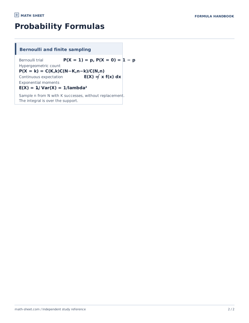
  • Weight the values by probabilityDiscrete: E[X] = Σi xi P(X = xi). Continuous: E[X] = ∫−∞∞ x f(x) dx.Use the density f for a continuous variable. The expectation is finite if the absolute first moment is finite.

    What it does

    Expected value is a probability-weighted mean. Sum over point masses or integrate against a density.

    Worked example

    Find the means of X taking values 0 and 4 with probabilities 1/4 and 3/4, and Y uniform on [0,4].

    1. For X, multiply and add: 0(1/4) + 4(3/4) = 3.
    2. For Y, integrate y/4 from 0 to 4: [y²/8] gives 2.
    Link to this example
  • Mean square distance and its rootVar(X) = E[(X − μ)²] = E[X²] − μ², σ = √Var(X)μ = E[X]. Use a finite second moment.

    What it does

    Variance is mean squared distance from the mean, and standard deviation is its nonnegative square root.

    Worked example

    X takes 2 or 6, equally likely. Find its variance and standard deviation.

    1. The mean is 4. Both values have squared distance 4 from it.
    2. The variance is 4 and the standard deviation is 2.
    Link to this example
  • Shift and scale XE[aX + b] = aE[X] + b, Var(aX + b) = a² Var(X)a and b are constants.

    What it does

    An additive shift moves the mean without changing spread. A scale a multiplies the mean by a and the variance by a².

    Worked example

    If E[X] = 3 and Var(X) = 4, find the mean and variance of Y = −2X + 5.

    1. E[Y] = −2(3) + 5 = −1.
    2. Var(Y) = (−2)²(4) = 16.
    Link to this example
See Statistics Formula Sheet

Models for counts and repeated trials

  • One yes-or-no trialP(X = 1) = p, P(X = 0) = 1 − pX is Bernoulli with success probability p.

    What it does

    A Bernoulli variable uses 1 for success with probability p and 0 for failure with probability 1 − p.

    Worked example

    Code a penalty kick as 1 for a goal and 0 otherwise. The chance of a goal is 0.7. Find both probabilities.

    1. By definition P(X = 1) = 0.7.
    2. Its complement is P(X = 0) = 0.3.
    Link to this example
  • Successes in n independent trialsP(X = k) = C(n,k)pk(1 − p)n−k, E[X] = np, Var(X) = np(1 − p)The binomial model uses k = 0, …, n and the same p for every trial.

    What it does

    The binomial distribution counts successes in a fixed number of independent trials with one common success probability.

    Worked example

    For four fair coin tosses, find P(exactly three heads), the mean and the variance.

    1. There are C(4,3) = 4 head positions, each with probability (1/2)⁴. Thus P = 1/4.
    2. The mean is 4(1/2) = 2. The variance is 4(1/2)(1/2) = 1.
    Link to this example
  • Trial index of the first successP(X = k) = (1 − p)k−1pThe geometric model assumes independent trials with fixed p > 0. Start at k = 1.

    What it does

    The geometric distribution counts trials up to and including the first success when trials are independent with constant success probability.

    Worked example

    A trial succeeds with probability 1/4. Find the chance of first success on trial 3.

    1. The first two trials must fail and the third must succeed.
    2. Multiply (3/4)²(1/4) = 9/64.
    Link to this example
  • Poisson count in a fixed intervalP(X = k) = e−λλk/k!k = 0, 1, 2, … and λ > 0 is the mean count over the interval.

    What it does

    A Poisson model gives integer count probabilities from a positive average count λ over the interval.

    Worked example

    A count is Poisson with mean 2. Find the probability of exactly one occurrence.

    1. Use λ = 2 and k = 1 in the mass formula.
    2. The probability is e−22/1! = 2e−2 ≈ 0.2707.
    Link to this example
  • Successes in a sample without replacementP(X = k) = C(K,k)C(N − K,n − k)/C(N,n)There are K successes among N objects. Choose n uniformly without replacement. A feasible k satisfies max(0,n + K − N) ≤ k ≤ min(n,K).

    What it does

    The hypergeometric distribution counts successes when drawing uniformly without replacement from a finite population.

    Worked example

    A group has 4 red and 6 blue tokens. Draw 3 without replacement. Find the chance of exactly 2 red.

    1. Choose 2 of the 4 red and 1 of the 6 blue. There are 6 × 6 = 36 such sets.
    2. There are C(10,3) = 120 total sets, so P = 36/120 = 0.3.
    Link to this example
See AP Statistics Formula Sheet

Densities for continuous measurements

  • Uniform density on an intervalf(x) = 1/(b − a) for a ≤ x ≤ b, and 0 elsewhere.Take a < b.

    What it does

    A uniform density has constant height over its interval, so a subinterval probability is its share of the total length.

    Worked example

    If X is uniform on [2,10], find P(4 ≤ X ≤ 7).

    1. The density is 1/(10 − 2) = 1/8 on the interval.
    2. Multiply by the subinterval length 7 − 4 = 3 to get 3/8.
    Link to this example
  • Normal density and standardizationf(x) = exp[−(x − μ)²/(2σ²)]/[σ√(2π)], Z = (X − μ)/σFor σ > 0, Z from this normal model has mean 0 and standard deviation 1.

    What it does

    A normal density is centered at μ and spread by σ. A z-score expresses an observation’s signed distance from μ in standard deviations.

    Worked example

    A normal variable has mean 50 and standard deviation 5. Find the z-score of 60 and the density at the mean.

    1. For 60, z = (60 − 50)/5 = 2.
    2. At 50 the exponential factor is 1, so the density is 1/[5√(2π)].
    Link to this example
  • Exponential waiting timef(x) = λe−λx for x ≥ 0 and 0 otherwise, E[X] = 1/λ, Var(X) = 1/λ²λ > 0. For any density, integrate over an interval to find its probability.

    What it does

    The exponential density models nonnegative waiting time at a constant event rate λ. Its mean is 1/λ and its variance is 1/λ².

    Worked example

    A waiting time is exponential with rate 2 per hour. Find its mean, variance and chance of waiting more than an hour.

    1. The mean is 1/2 hour and the variance is 1/4 hour².
    2. Integrating 2e−2x from 1 to infinity gives e−2, about 0.1353.
    Link to this example

Preview the printable

Download the compact sheet for a quick review, or print the complete formula list from this page.

Practice these skills

Related references

Sources and review

Math Sheet prepares original print materials. See how we check formulas and printouts.

Browse all formula sheets →