
Preview page 2
2 pages · US Letter / A4
Statistics Formula Sheet
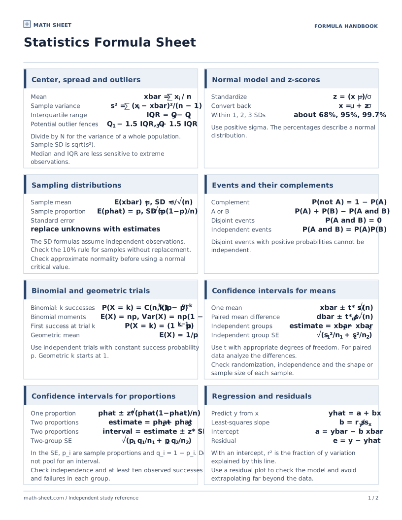
Printable statistics formula sheet with descriptive statistics, z-scores, sampling distributions, confidence intervals, test statistics and regression.
Introductory statistics
Choose a calculation by the job: describe a data set, model a random outcome, estimate a parameter or check a claim. Keep the assumptions near the formula when you work.
On this page
Open a formula for its definition and a worked example.
Statistics Formula Sheet
What it does
The sample mean divides the total of all observations by their count. Every observation contributes equally.
Worked example
Find the mean of 3, 5, 8, 12.
What it does
Population variance averages squared deviations from the population mean. Its square root restores the original units.
Worked example
Treat 1, 3, 5 as an entire population. Find variance and standard deviation.
What it does
Sample variance estimates population variance by dividing squared deviations from the sample mean by n − 1. Sample standard deviation is its square root.
Worked example
Treat 2, 4, 6 as a sample. Find s² and s.
What it does
The interquartile range is the difference between the upper and lower quartiles. It measures the spread of the central half of the data.
Worked example
A data set has Q₁ = 12, median = 19, and Q₃ = 27. Find the IQR.
What it does
A z-score gives the signed distance from the mean in standard deviations. A positive standard deviation is required.
Worked example
A score of 64 comes from a distribution with mean 70 and standard deviation 4. Find z.
What it does
Complementary events partition the outcomes. The inclusive union adds the event probabilities and subtracts the overlap once.
Worked example
If P(A) = 0.4, P(B) = 0.5, and P(A ∩ B) = 0.2, find P(Aᶜ) and P(A ∪ B).
What it does
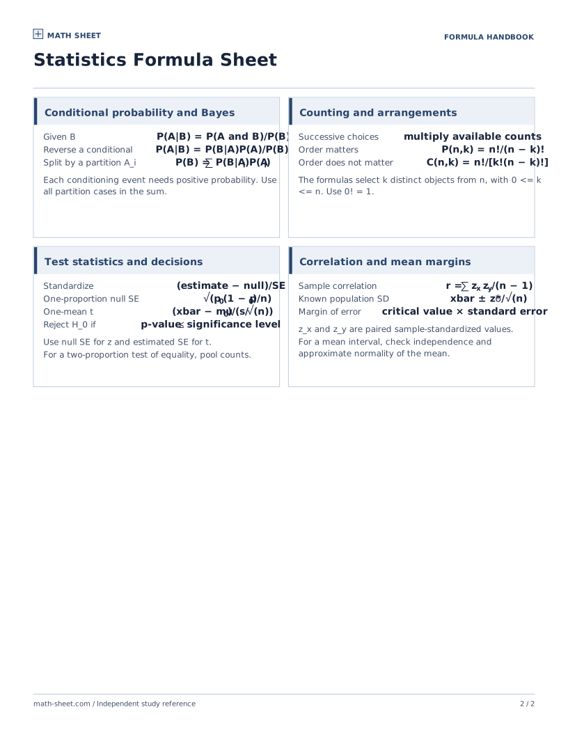
Conditioning restricts attention to an event of positive probability. The multiplication rule recovers a joint probability from a marginal and a conditional probability.
Worked example
Of 40 students, 20 take art, 10 take music, and 5 take both. Find P(art | music) and P(both).
What it does
Bayes’ theorem updates a prior event probability when an observation occurs by multiplying by the observation likelihood and dividing by its overall probability.
Worked example
Line A makes 60% of bulbs with 2% defective. Line B makes 40% with 5% defective. A bulb is defective. Find P(A | defective).
What it does
A permutation counts ordered selections of distinct objects. A combination ignores order by dividing by the number of arrangements of the chosen objects.
Worked example
From five people, count two-person teams and ordered president–vice-president assignments.
What it does
The binomial probability counts the placements of k successes among n independent trials and multiplies by the probability of one such placement.
Worked example
A fair coin is tossed four times. Find the probability of exactly two heads.
What it does
A binomial count has mean np and variance np(1 − p), because independent trial outcomes contribute their means and variances additively.
Worked example
Find the mean and standard deviation for 20 independent trials with p = 0.25.
What it does
For a normal distribution, approximately 68%, 95%, and 99.7% of observations lie within one, two, and three standard deviations of the mean.
Worked example
A normally distributed measurement has μ = 50 and σ = 3. What proportion lies between 44 and 56?
What it does
With known population standard deviation and an approximately normal sampling distribution, a z interval adds and subtracts the critical value times the standard error.
Worked example
A random independent sample has n = 64 and x̄ = 40. Assume σ = 8. Use z* = 1.96 for a 95% interval.
What it does
A one-sample t interval substitutes the sample standard deviation and uses a t critical value with n − 1 degrees of freedom. Check independence and sampling-distribution conditions.
Worked example
A random sample of 25 observations from an approximately normal population has x̄ = 18 and s = 5. Use t* = 2.064.
What it does
The large-sample normal interval for a proportion uses p̂ to estimate its standard error. Check independence and that both outcome counts are sufficiently large.
Worked example
In 100 independent observations there are 40 successes. Use z* = 1.96 for a 95% interval.
What it does
The least-squares line with intercept has slope equal to correlation times the ratio of sample standard deviations. It passes through the pair of sample means.
Worked example
Given r = 0.75, sx = 2, sy = 4, x̄ = 5, and ȳ = 12, predict y at x = 7.
What it does
Pearson correlation averages products of paired sample-standardized values with divisor n − 1. Both variables need positive sample spread.
Worked example
Find r for paired observations (1, 4), (2, 2), and (3, 0).
What it does
For one-predictor least squares with an intercept, the fraction of response variation explained by the line equals the square of Pearson correlation.
Worked example
A least-squares line with intercept has r = −0.8. Find and interpret R².
Download the compact sheet for a quick review, or print the complete formula list from this page.
2 pages · US Letter / A4
Printable statistics formula sheet with descriptive statistics, z-scores, sampling distributions, confidence intervals, test statistics and regression.
Math Sheet prepares original print materials. See how we check formulas and printouts.