Calculus I–II

Integral Table and Integration Formulas

Match the integrand to a pattern, then check its domain. Use this table for standard antiderivatives and for deciding when substitution, integration by parts or a rational decomposition can simplify an integral.

On this page

Find a formula

Open a formula for its definition and a worked example.

Antiderivatives and accumulation

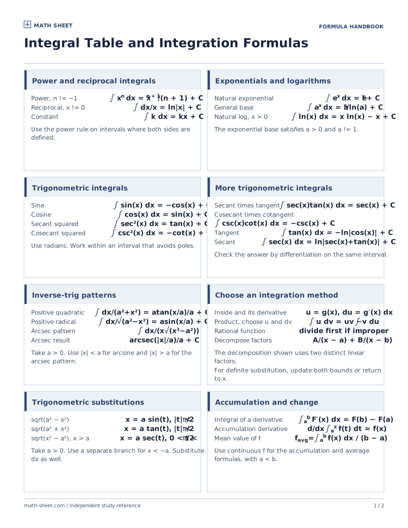
  • Raise the exponent by one∫ xn dx = xn+1/(n+1) + C, n ≠ −1Use an interval where the power is real and the antiderivative rule applies.

    What it does

    The power rule reverses the derivative of a power on intervals where the expression is defined. The exponent −1 uses a logarithm.

    Worked example

    Find ∫ x⁴ dx.

    1. Raise the exponent from 4 to 5 and divide by 5.
    2. The antiderivative is x⁵/5 + C.
    Link to this example
  • Reciprocal antiderivative∫ dx/x = ln|x| + CWork on an interval that excludes zero.

    What it does

    The derivative of ln|x| equals 1/x on either side of zero, with a separate integration constant on each interval.

    Worked example

    Find ∫ 3/x dx for x < 0.

    1. Take the factor 3 outside the integral.
    2. The result is 3 ln|x| + C, which equals 3 ln(−x) + C on this interval.
    Link to this example
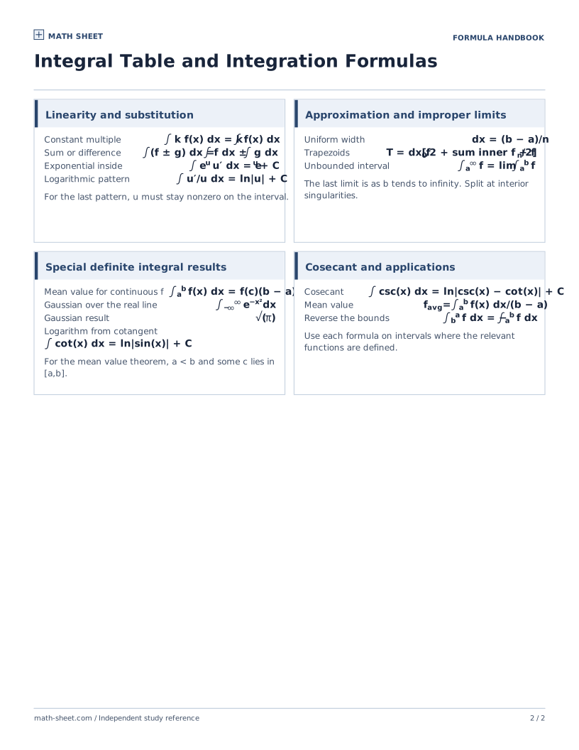
  • Integrate term by term∫ [αf(x) + βg(x)] dx = α∫ f(x) dx + β∫ g(x) dxα and β are constants. Keep one arbitrary constant in the result.

    What it does

    Linearity lets you integrate each term separately and carry constant multipliers through the integral.

    Worked example

    Find ∫ (6x² − 4x) dx.

    1. The first term integrates to 6x³/3 = 2x³.
    2. Subtract 4x²/2 and add one constant: 2x³ − 2x² + C.
    Link to this example
  • Evaluate at the endpoints∫ab F′(x) dx = F(b) − F(a)This holds when F′ is continuous on the integration interval.

    What it does

    A definite integral of a continuous derivative gives the function’s net change from the lower endpoint to the upper endpoint.

    Worked example

    Evaluate ∫13 2x dx.

    1. The function F(x) = x² has derivative 2x.
    2. The net change is F(3) − F(1) = 9 − 1 = 8.
    Link to this example

Exponential and logarithmic patterns

  • Integrate a constant base to the x∫ ex dx = ex + C, ∫ ax dx = ax/ln a + CFor the second rule, a > 0 and a ≠ 1.

    What it does

    Exponentials reproduce themselves under differentiation up to the factor ln a. Integrating divides out that factor.

    Worked example

    Integrate 2x + ex.

    1. For 2x, divide by ln 2. For ex, the factor is ln e = 1.
    2. The result is 2x/ln 2 + ex + C.
    Link to this example
  • Exponential with its inner derivative∫ eu u′ dx = eu + CHere u is a differentiable function of x.

    What it does

    An exponential of an inner function integrates to that same exponential when the inner derivative is a factor.

    Worked example

    Find ∫ 6x e3x² dx.

    1. Set u = 3x², so du = 6x dx.
    2. Integrate eu to get e3x² + C.
    Link to this example
  • Integrate the natural logarithm∫ ln x dx = x ln x − x + CFor x > 0. This follows by integrating by parts.

    What it does

    The natural log integrates by parts, taking its derivative 1/x and integrating the other factor 1.

    Worked example

    Evaluate ∫1e ln x dx.

    1. Integration by parts gives F(x) = x ln x − x for x > 0.
    2. F(e) − F(1) = 0 − (−1) = 1.
    Link to this example
  • A denominator and its derivative∫ (u′/u) dx = ln|u| + CUse an interval where u is differentiable and never zero.

    What it does

    A quotient with the derivative of its denominator on top integrates to the log of the denominator’s absolute value.

    Worked example

    Integrate 8x/(4x² + 5).

    1. The derivative of 4x² + 5 is 8x.
    2. The denominator is always positive, so the result is ln(4x² + 5) + C.
    Link to this example

Trig antiderivatives

  • Sine and cosine∫ sin x dx = −cos x + C, ∫ cos x dx = sin x + C

    What it does

    The derivatives of sin x and −cos x are cos x and sin x respectively, with angles measured in radians.

    Worked example

    Integrate 3 sin x − 2 cos x.

    1. The sine term contributes −3 cos x.
    2. The cosine term contributes −2 sin x, giving −3 cos x − 2 sin x + C.
    Link to this example
  • Squared secant and cosecant∫ sec² x dx = tan x + C, ∫ csc² x dx = −cot x + C

    What it does

    The squared trig reciprocals are derivatives of tangent and negative cotangent where those functions exist.

    Worked example

    Integrate 2 sec² x + 5 csc² x on 0 < x < π/2.

    1. The secant term integrates to 2 tan x.
    2. The cosecant term integrates to −5 cot x, giving 2 tan x − 5 cot x + C.
    Link to this example
  • Products with matching derivatives∫ sec x tan x dx = sec x + C, ∫ csc x cot x dx = −csc x + C

    What it does

    The products sec x tan x and csc x cot x differentiate back from sec x and −csc x respectively.

    Worked example

    Integrate sec x tan x − 2 csc x cot x on 0 < x < π/2.

    1. The first antiderivative is sec x. The second term has antiderivative 2 csc x.
    2. Their sum is sec x + 2 csc x + C.
    Link to this example
  • Tangent and cotangent∫ tan x dx = −ln|cos x| + C, ∫ cot x dx = ln|sin x| + C

    What it does

    Tangent and cotangent can be written as a derivative divided by a trig function, which produces a logarithm.

    Worked example

    Integrate tan x + cot x on 0 < x < π/2.

    1. The tangent term gives −ln(cos x). The cotangent term gives ln(sin x).
    2. Combine them as ln(tan x) + C on this interval.
    Link to this example
  • Secant and cosecant alone∫ sec x dx = ln|sec x + tan x| + C, ∫ csc x dx = ln|csc x − cot x| + CUse radians and stay within an interval where the integrand is defined.

    What it does

    Secant and cosecant alone have logarithmic antiderivatives. The absolute values allow any interval where the integrands are defined.

    Worked example

    Integrate sec x on [0,π/4] and csc x on [π/4,π/2].

    1. For sec x, evaluate ln|sec x + tan x| at the endpoints: ln(√2 + 1) − ln 1 = ln(√2 + 1).
    2. For csc x, evaluate ln|csc x − cot x|: ln 1 − ln(√2 − 1) = ln(√2 + 1).
    Link to this example
See Trigonometry Formula Sheet

Spot an inverse-trig derivative

  • Square root of a difference∫ dx/√(a² − x²) = arcsin(x/a) + Ca > 0 and |x| < a.

    What it does

    A reciprocal square root of a² − x² integrates to an arcsine on the interval |x| < a for a > 0.

    Worked example

    Integrate 1/√(25 − x²) for −5 < x < 5.

    1. Match a² = 25, so a = 5.
    2. The result is arcsin(x/5) + C.
    Link to this example
  • Sum of squares∫ dx/(a² + x²) = arctan(x/a)/a + Ca > 0.

    What it does

    The derivative of arctan(x/a) gives a/(a² + x²). Dividing by a produces the desired reciprocal.

    Worked example

    Integrate 1/(16 + x²).

    1. Use a = 4 because 16 = 4².
    2. The result is arctan(x/4)/4 + C.
    Link to this example
  • Product with a difference of squares∫ dx/[x√(x² − a²)] = arcsec(|x|/a)/a + Ca > 0 and |x| > a. Equivalently use arccos(a/|x|)/a + C.

    What it does

    The arcsecant form applies to the reciprocal of x√(x² − a²) on either interval |x| > a.

    Worked example

    Integrate 1/[x√(x² − 9)] for x > 3.

    1. Take a = 3, and here |x| = x.
    2. The result is arcsec(x/3)/3 + C, or arccos(3/x)/3 + C.
    Link to this example

Rewrite before integrating

  • Reverse the chain ruleu = g(x), du = g′(x) dx, ∫ f(g(x))g′(x) dx = ∫ f(u) duFor a definite integral, also convert the bounds to u.

    What it does

    Substitution combines a composite function with its inner derivative to turn an integral in x into a simpler integral in u.

    Worked example

    Evaluate ∫01 2x(1 + x²)³ dx.

    1. Let u = 1 + x². Then du = 2x dx, and u goes from 1 to 2.
    2. Evaluate [u⁴/4] from 1 to 2 to get (16 − 1)/4 = 15/4.
    Link to this example
  • Integration by parts∫ u dv = uv − ∫ v du

    What it does

    Integration by parts reverses the product rule. Choose u to simplify upon differentiation and dv to integrate easily.

    Worked example

    Find ∫ x cos x dx.

    1. Take u = x and dv = cos x dx, so du = dx and v = sin x.
    2. Then ∫ x cos x dx = x sin x − ∫ sin x dx = x sin x + cos x + C.
    Link to this example
  • Choose a trig substitution for the radical√(a² − x²): x = a sin θ. √(a² + x²): x = a tan θ. √(x² − a²): x = a sec θ.Use a > 0 and select an angle interval consistent with the sign of x and the radical.

    What it does

    Trig substitution replaces a radical with a simpler trig expression by matching a Pythagorean identity to the signs in the radicand.

    Worked example

    Simplify √(9 − x²) for 0 ≤ x < 3, √(9 + x²) for x ≥ 0, and √(x² − 9) for x ≥ 3.

    1. Use x = 3 sin θ for the first and x = 3 tan θ for the second. They simplify to 3 cos θ and 3 sec θ on 0 ≤ θ < π/2.
    2. For x ≥ 3 use x = 3 sec θ on the same angle range. The third radical becomes 3 tan θ.
    Link to this example
  • Split distinct linear denominator factorsP(x)/[(x − a)(x − b)] = A/(x − a) + B/(x − b)Requires a ≠ b and degree P < 2. For a higher degree numerator, divide first.

    What it does

    A proper rational function with two distinct linear denominator factors splits into two constant-over-linear fractions.

    Worked example

    Decompose 1/[(x − 1)(x + 2)].

    1. After multiplying through, 1 = A(x + 2) + B(x − 1). Set x = 1 and x = −2.
    2. A = 1/3 and B = −1/3. The split is 1/[3(x − 1)] − 1/[3(x + 2)].
    Link to this example
See Derivatives cheat sheet

Definite integrals with special interpretations

  • Extend the upper bound without limit∫a∞ f(x) dx = limR→∞ ∫aR f(x) dxThe improper integral converges if this limit is finite. Split at any interior singularity.

    What it does

    An integral to infinity converges when the integral up to a finite cutoff tends to a finite number.

    Worked example

    Evaluate ∫1∞ x−2 dx.

    1. For cutoff R, the integral is [−1/x] from 1 to R, which is 1 − 1/R.
    2. As R → ∞ it converges to 1.
    Link to this example
  • Average value and where it occursfavg = [1/(b − a)] ∫ab f(x) dx. If f is continuous, f(c) = favg for some c ∈ [a,b].Take a < b.

    What it does

    The average value is area with sign divided by interval length. A continuous function attains that average somewhere on the interval.

    Worked example

    Find the average of f(x) = x² on [0,3] and a point where it occurs.

    1. The integral is [x³/3] from 0 to 3 = 9. Divide by 3 to get average 3.
    2. Solve c² = 3 on [0,3], giving c = √3.
    Link to this example
  • Area under the Gaussian bell∫−∞∞ e−x² dx = √π

    What it does

    The Gaussian integral supplies the total area of e−x². Rescaling its input rescales the area by the reciprocal of the positive scale factor.

    Worked example

    Evaluate ∫−∞∞ e−4x² dx.

    1. Let u = 2x so dx = du/2, with bounds still running over the whole line.
    2. The result is half the basic Gaussian integral, or √π/2.
    Link to this example
See Limits Cheat Sheet

Preview the printable

Download the compact sheet for a quick review, or print the complete formula list from this page.

Practice these skills

Related references

Sources and review

Math Sheet prepares original print materials. See how we check formulas and printouts.

Browse all formula sheets →