
Probability
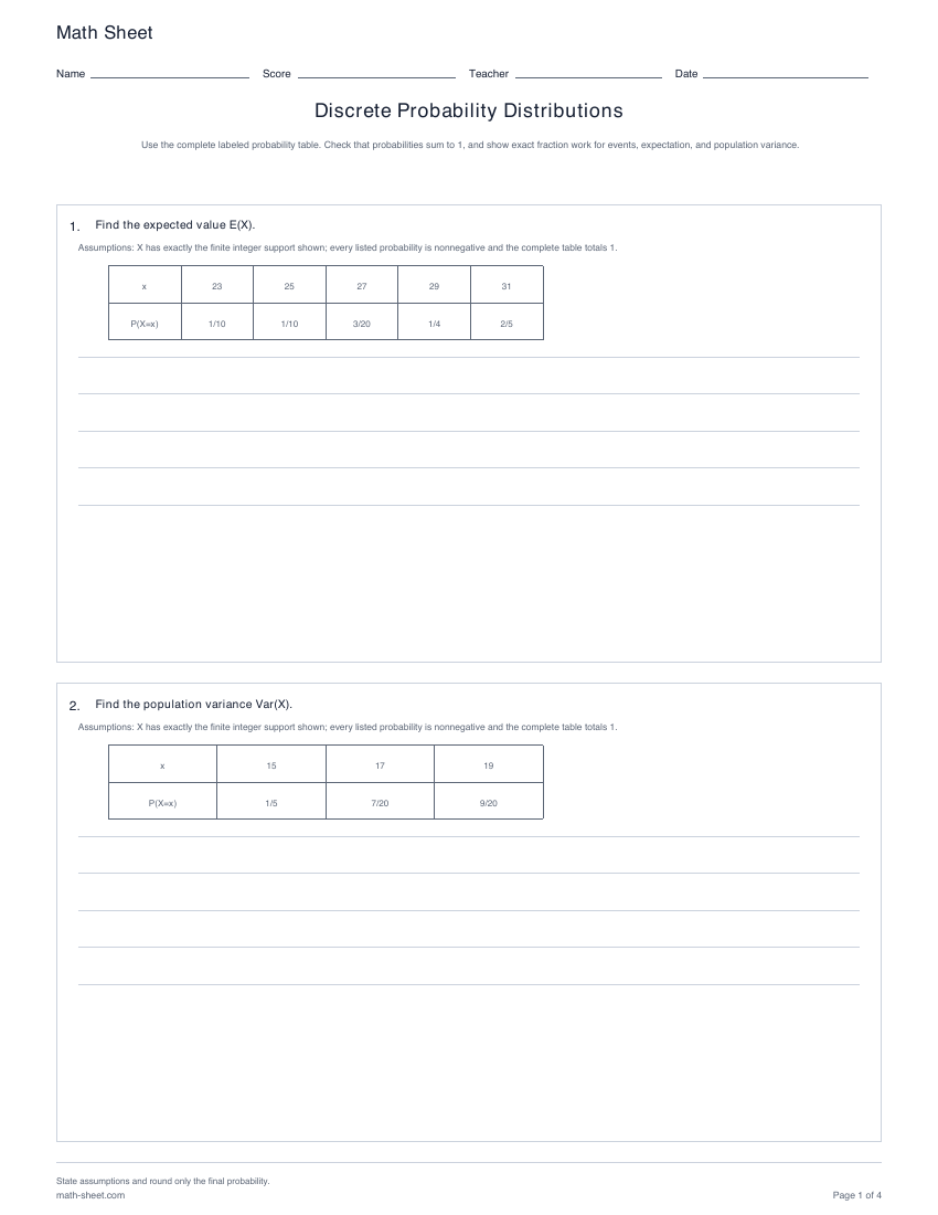
Discrete Probability Distributions worksheets
Use valid finite probability tables to find missing entries, event probabilities, expected value, and population variance.
Preview and downloadStatistics practice
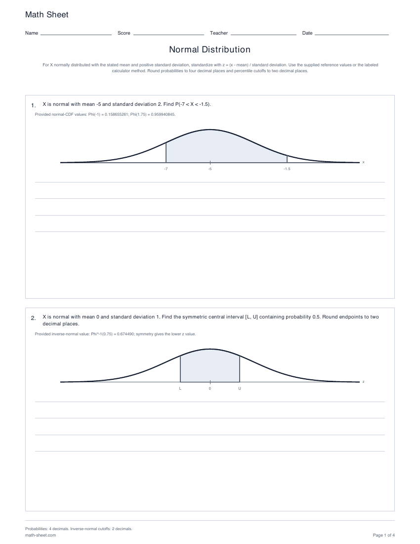
Standardize normal values, find below, above, and between probabilities, and invert the model for percentiles and central intervals.
Ready-made English PDF · fixed settings
Customization below makes a separate PDF.
Fixed English ready-made files. Custom settings below apply only to the configured PDF.
Ready to print
Write the normal model first. Standardize probability cutoffs before using Phi, and use inverse normal for requested cutoffs. Keep full precision during calculation, then round probabilities to four decimals and cutoffs to two decimals.
Download the practice pages alone, or include a separate answer key or teacher model. Longer activities may use more than one page.
Customize this worksheetEach problem starts with a complete normal model, including a positive standard deviation. Learners standardize printed cutoffs exactly, shade the matching tail or interval, and choose cumulative, survival, difference, or inverse-normal work to match the question.
Learning objective
Connect a stated normal model to z-scores, cumulative probability, upper tails, differences of cumulative probabilities, and inverse-normal cutoffs.
Worked example
Phi^-1(0.90) ≈ 1.2815516, so c = 50 + 10(1.2815516) ≈ 62.82.
The unknown is a cutoff, so invert the cumulative probability first and then undo standardization. Checking (62.82 − 50)/10 ≈ 1.282 gives a left-tail probability of about 0.9001; the small difference is rounding. About 10% lies above the cutoff.
Teaching notes
Write the mean and positive standard deviation before using the normal model. For a value x, standardize with z = (x − mean)/standard deviation. Phi(z) is the area to the left; upper tails use 1 − Phi(z), and intervals use the upper cumulative probability minus the lower one. Normal probabilities describe an assumed model, not a guarantee about every observed data set.
For example, when the mean is 50 and the standard deviation is 10, P(40 < X < 60) = Phi(1) − Phi(−1) ≈ 0.8413 − 0.1587 = 0.6826 using rounded table entries (0.6827 from full precision). A percentile reverses this workflow: a 90th-percentile cutoff uses Phi^-1(0.90), not Phi(0.90). For a central 90% interval, the remaining 10% splits into 5% per tail, so use the 0.05 and 0.95 quantiles.
The worksheets support below, above and between probabilities, inverse percentiles and central intervals. Begin with shaded sketches, then mix area and cutoff tasks to assess method choice. Teachers can print Letter or A4 with a separate worked key. Keep full precision until the requested final rounding; broader model selection and nonnormal inference require other resources.
No. Here the scale parameter is the positive standard deviation. If a course writes N(μ, σ²), its second parameter is variance; take its square root before using z = (x − μ)/σ.
Use cumulative area 0.90 because 90% lies below the cutoff and 10% above it. For mean 50 and standard deviation 10 this gives approximately 62.82.
Make it yours
Choose your options, update the preview, then download the exact same pages.
Choose probability, percentile, or central-interval tasks; general or standard models; a self-contained reference or calculator-required sheet; and a reproducible seed.
A useful next step
Probability
Use valid finite probability tables to find missing entries, event probabilities, expected value, and population variance.
Preview and download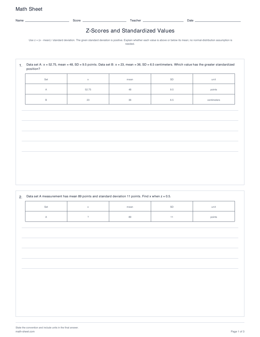
Statistics
Calculate z-scores, recover original values, and compare relative positions across data sets with positive standard deviations.
Preview and download